SQL Server Window Functions: An introduction for beginners

Window functions in SQL Server are very powerful tools we can use to gather meaningful information from our database.

Window functions are considered an advanced tool when querying data in SQL Server. If you’re trying to learn about window functions, congratulations, you’re moving up!

Do you need to understand how window functions work in SQL Server? You’ve come to the right place!

In this tutorial, we’re going to discuss the basics of window functions in SQL Server. This tutorial is meant to be an introduction to window functions. In the coming weeks, we’ll dive deeper into all the functions and give you all the juicy details you need to know.

Also, make sure you download your FREE Ebook:

FREE Ebook on SQL Server Window Functions!

This FREE EBook discusses absolutely everything you need to know about window functions in SQL Server, including everything discussed in this tutorial. This eBook will definitely be a great resource for you to reference throughout your career as a data professional. Get it today!

Here are the topics we’ll discuss:

1. What is a window function?
2. What is a ‘window’ anyway?
3. The parts to a window query
4. Understanding the window frame
5. Tips, tricks, and links

Let’s do it.

1. What is a window function?

A window function can be used to combine aggregate/ranking/offset information AND detail information in a single query.

Window functions are excellent for writing a single query that shows grouped information AND individual information in a single query. If you think about it, you would normally use the GROUP BY clause to show grouped information, which is fine. But the GROUP BY query has it’s limits, in that it won’t show you individual data also.

Setting up some data

We need to set up some good data to work through this tutorial. We’ll create a Customers, Products, and Orders table and populate them with information. You’ll want to do this to make sure you can follow along:

First, we’ll create and populate the Customers table:

--Create Customers table
CREATE TABLE Customers
(
CustID INT PRIMARY KEY IDENTITY(50,5),
FirstName VARCHAR(20),
LastName VARCHAR(20)
)

--Populate Customers table with data
INSERT INTO Customers(FirstName, LastName)
VALUES
('Joshua','Porter'),
('Andrew','Bluefield'),
('Jack','Donovan'),
('Cindy','Thatcher'),
('Gordon','Acres'),
('Gretchen','Hamilton')

Now the Products table:

--Create Products table
CREATE TABLE Products
(
ProductID INT PRIMARY KEY IDENTITY(20,2),
ProductName VARCHAR(20),
Price DECIMAL(5,2)
)

--Populate Products table with data
INSERT INTO Products (ProductName, Price)
VALUES
('Large Bench',198.00),
('Small Bench',169.40),
('Coffee Table',220.00),
('Side Tables',265.20),
('Coat Rack',45.00)

Now the Orders table:

--Create Orders table
CREATE TABLE Orders
(
OrderID INT PRIMARY KEY IDENTITY(100,10),
CustID INT,
ProdID INT,
Qty TINYINT,
Orderdate DATETIME
)

--Populate Orders table with data
INSERT INTO Orders(CustID, ProdID, Qty, Orderdate)
VALUES
(55, 22, 1, '6/1/2021'),
(60, 28, 2, '6/6/2021'),
(75, 26, 1, '6/13/2021'),
(50, 20, 1, '7/1/2021'),
(55, 28, 1, '7/6/2021'),
(65, 24, 1, '7/14/2021'),
(55, 26, 1, '7/18/2021'),
(50, 26, 1, '7/24/2021'),
(70, 24, 1, '8/6/2021'),
(70, 26, 1, '8/6/2021'),
(70, 22, 3, '9/1/2021')

Awesome. Notice all the tables use the IDENTITY property to automatically populate the primary key columns on inserts. Very handy thing to use.

Read more: IDENTITY Column in SQL Server: Everything you need to know

Also notice the Orders table contains unofficial foreign key links to the Customers and Products tables. I say they are “unofficial” because I didn’t actually create a foreign key constraint between the tables. It’s not necessary for this tutorial.

Read more about foreign key constraints: SQL Server Foreign Key: Everything you need to know

Let’s run a quick query with a couple of JOINS to see all the data laid out nicely for us:

SELECT C.CustID, C.FirstName, C.LastName, P.ProductName, P.Price as 'Product Price', 
O.Qty, O.OrderDate
FROM Orders as O
INNER JOIN Customers AS C
ON O.CustID = C.CustID
INNER JOIN Products as P
ON O.ProdID = P.ProductID

This query will give us the following result:

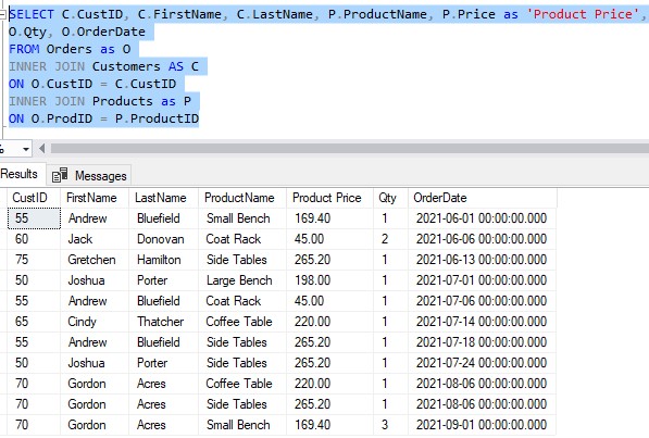
Nice. In this result set, we can see some really great details about each order. We can see the following details:

• Who made the order
• What they bought
• How much that product costs
• How many of that product they bought
• The date they made the order

I mentioned earlier how there are some limitations to the GROUP BY clause. Let’s look at an example.

Limitations of a GROUP BY query

In the result set above, what if I wanted to know how much each customer has spent at our store?

Normally, that would be a simple GROUP BY query. Let’s add an aggregate to our SELECT list, then add a GROUP BY clause to give us a breakdown for each customer (spoiler alert: this query won’t run):

SELECT C.CustID, C.FirstName, C.LastName, P.ProductName, P.Price as 'Product Price', 
O.Qty, O.OrderDate,
SUM(P.Price*o.Qty) as CustomerTotal
FROM Orders as O
INNER JOIN Customers AS C
ON O.CustID = C.CustID
INNER JOIN Products as P
ON O.ProdID = P.ProductID
GROUP BY C.CustID

We get the following error message when we try to run this query:

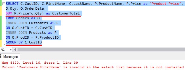
The error message is complaining because there are columns in our SELECT list that are not within our GROUP BY clause.

Read more about the GROUP BY clause: GROUP BY clause: A How-To Guide

So how would we get the information we want using a GROUP BY clause? Remember, we want to know how much money each customer has spent with us.

Well, we would need to strip away many of the columns in our query. Try this:

SELECT C.CustID, C.FirstName, C.LastName,
SUM(P.Price*O.Qty) as CustomerTotal
FROM Orders as O
INNER JOIN Customers AS C
ON O.CustID = C.CustID
INNER JOIN Products as P
ON O.ProdID = P.ProductID
GROUP BY C.CustID, C.FirstName, C.LastName

This will give us the following results:

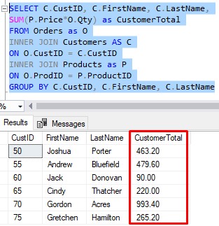
Great…

But now, many of those details we saw earlier are long gone. I was able to add the customer’s first and last name to the result set, but what about details about the products they bought? Those details are long gone. And what about details of the order, like the quantity of the item purchased and the order date? You guessed it, those are long gone.

Window functions can show us detail AND aggregate information

Through the use of a window function, we can keep all those details, while also displaying aggregate information, too. Check it out (I’m purposefully not showing you the query yet. We’ll figure it out together):

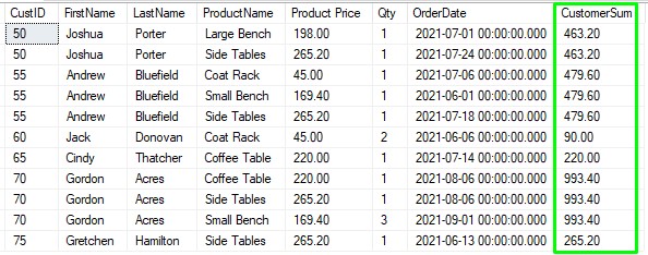
Let’s look at the first customer, Joshua Porter. It looks like he bought two items from us, the “Large Bench” and the “Side Tables”. If we multiply each price by the quantity (which is just 1 for each), then add the numbers together, we calculate that Joshua Porter has spent a grand total of $463.20 at our store, which is exactly what we see in our new CustomerSum column! The number is repeated for each row for Joshua, but that’s ok.

Same story is true for the next customer, Andrew Bluefield. If we add up everything he has bought, it comes to $479.60, which is what we have in our new column! (again, the number is repeated for each row for Andrew, but that’s ok!)

I challenge you to double-check each customer. Don’t forget to multiply the price by the quantity!

Remember, the point is that we can see all those great details about the customers, products, and orders AND aggregate information. We’ll also talk about how you can also see ranking and offset information if you need to.

2. What is a “window” anyway?

A window is basically just a set of rows. We outline the set of rows we want in the window by using an OVER clause.

In fact, that’s the first step to using a window function: Specifying an OVER clause. The OVER clause is basically the heart of a window function query.

So let’s start with that. We write our aggregate function (which is SUM(P.Price*O.Qty)), then specify an OVER clause next to it:

SELECT C.CustID, C.FirstName, C.LastName, P.ProductName, P.Price as 'Product Price', 
O.Qty, O.OrderDate,
SUM(P.Price*O.Qty) OVER () as Total
FROM Orders as O
INNER JOIN Customers AS C
ON O.CustID = C.CustID
INNER JOIN Products as P
ON O.ProdID = P.ProductID

Notice the OVER clause has parentheses next to it. Within those parentheses, you can specify lots of information (of which we will soon see) or you can simply choose to leave them empty like we have done.

So remember, the OVER clause specifies the set of rows we want within our window. But if the OVER clause is empty, what will the set of rows be?

Answer: The window will contain all rows in the result set.

The SUM aggregate function is applied to all rows in the result set. In other words, the query above is going to show us the grand total of everything that has been purchased by EVERYONE. Again, since the OVER clause is empty, we’re working with all rows in our result set:

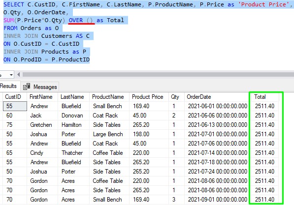
I challenge you to check the math. Again, don’t forget about the quantities.

(I double-checked, and yes, the grand total of everything that has been purchased by everyone is $2511.40)

Like before, the number is repeated for every row, but that’s ok!

How to ‘partition’ in a window function

Remember what we wanted to see earlier. We wanted to see a breakdown by Customer. We wanted to know how much each customer has spent at our store.

If that’s what we want, we need to specify a different window. We don’t want one GIANT window anymore. Instead, we want one window per customer. Each window will contain rows for just that customer.

The concept is similar to when you use the GROUP BY clause. In your OVER clause, you can specify how you want the data to be grouped.

In the OVER clause, the way we specify groups is to use the PARTITION BY clause. For our example, the best way to identify each customer is by their CustID. So, that’s what we outline in our query:

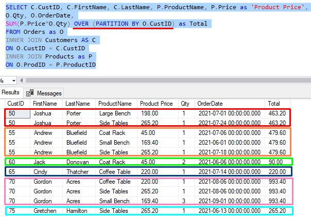
Now, each CustID is in it’s own window. The SUM aggregate function is applied to only the rows in each window.

For example, first we calculate the sum for Joshua Porter, and get $463.20. 

But then we move on to a different customer, Andrew Bluefield. Since his rows are in his own window, his sum will obviously be different. His sum is $479.60.

The process continues for each CustID. We continue to get a breakdown per CustID.

Pretty neat, right?

3. The parts to a window query

To understand all the parts to a window query, we need to think about another example of a query we would like to see.

What if we wanted to see a running total of customer purchases? Meaning we want to see how much money each customer had spent at our store at that point in time?

Take a look at our query without any window functions:

Let’s look at the orders for Andrew Bluefield, for example. He bought his items on the following dates:

• 6/1/2021
• 7/6/2021
• 7/18/2021

Wouldn’t it be nice to know how much money he had spent with us at each of those points in time? For example, the first time Andrew bought anything from us was on 6/1/2021. At that point in time, he had only spent $169.40 with us (which is the cost of the product he bought on that day, of course).

On 7/6/2021, he bought another product from us, which was the coat rack for $45.00. So again, at that point in time, the total amount of money he had spent with us was $45.00 plus the $169.40 he spent before. So his running total at THAT point in time was $214.40.

You still with me?

Finally, on 7/18/2021, he bought the Side Tables for $265.20. His running total (the sum of everything he has ever bought up to that point in time) is $479.60.

So, I guess we figured out his running total the hard way. Through the use of a window frame, we’ll see how SQL Server can calculate this same information for us.

The way we would get a running total for each customer is to write a query like this:

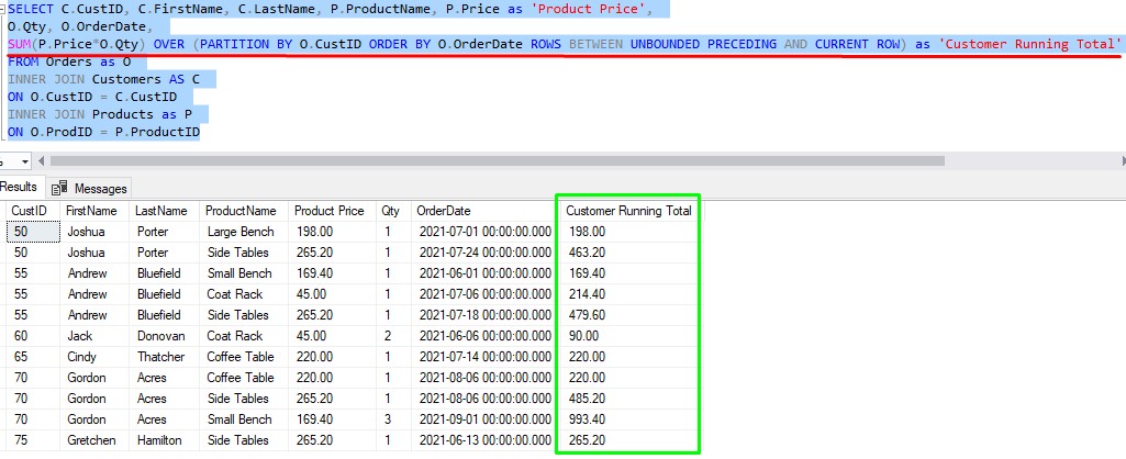
Here is a breakdown of all the parts of our window expression:

We need to talk about each part:

The window function itself

There are many window functions out there:

• Aggregate window functions – These are the same aggregate functions you would normally use with a GROUP BY query. All of these take some kind of argument, like they normally would when you use them in a GROUP BY query.
  • SUM
  • COUNT
  • MIN
  • MAX
  • AVG
• Ranking window functions – These allow you rank rows in your window, according to some ordering you specify. None of them take an argument except for NTILE which takes an integer as an argument.
  • ROW_NUMBER
  • RANK
  • DENSE_RANK
  • NTILE
• Offset window function – These tell you information about a row that is at the beginning or end of a window, or a row that is a specified offset from the current row. They all take one argument, which is the name of the element you want to return from the offset row.
  • FIRST_VALUE
  • LAST_VALUE
  • LAG
  • LEAD

I have a full tutorial on the different ranking window functions you should definitely read next:

SQL Server Ranking Window Functions: ROW_NUMBER, RANK, DENSE_RANK, NTILE

I also have a full tutorial on the different offset window functions:

SQL Server Offset Window Functions: FIRST_VALUE, LAST_VALUE, LAG, LEAD

The OVER clause

As I mentioned earlier, the OVER clause is the heart of a window function query. Every window function needs to have an OVER clause. As we saw earlier, sometimes it can be completely empty. Other times, it can be packed full of details, like in our “running total” example.

Window partition clause

We talked about this earlier. This basically identifies how you want to window your data. You use the PARTITION BY clause to identify how you want your data to be partitioned.

You can leave out a window partition clause which will put all rows in your result set into one large partition.

Window order clause

We’ll see that some window functions require a window order clause. The order clause is just the words “ORDER BY“, which you are probably familiar with. Of course, after the words “ORDER BY“, you specify the column(s) in which you want your data to be ordered.

Window frame clause

The frame clause is probably the most complex part of a window function. In your OVER clause, sometimes you’ll want to specify a window frame. A frame basically specifies a subset of rows within the window.

Some window functions don’t support a frame. For those that do, they require that you also specify a window order clause.

I’ll outline the keywords we can use for window frames, but they probably won’t make sense right now. We’ll talk about them and give you some examples in the next sections.

First, understand that there is something called a window frame unit. It can be either the keyword “ROWS” or the keyword “RANGE“.

With the ROWS unit, you can specify the following frame delimiters:

• UNBOUNDED PRECEDING – The beginning of the window
• UNBOUNDED FOLLOWING – The end of the window
• CURRENT ROW – The current row (window functions operate on a row-by-row basis)
• N PRECEDING – A specified number of rows before the current row
• N FOLLOWING  – A specified number of rows after the current row

With the RANGE unit, you can specify only some of the same delimiters mentioned above.

• UNBOUNDED PRECEDING
• UNBOUNDED FOLLOWING
• CURRENT ROW

I know, you don’t understand.

4. Understanding the window frame

Let’s look at the result set for Andrew Bluefield with a RunningTotal column. I purposefully erased the values in the column so that we could better understand the idea of a window frame:

As I mentioned earlier, window functions operate on a row-by-row basis, starting from the top and working their way down.

The first thing to point out is how these rows are ordered by OrderDate. This is the order in which Andrew bought items from our store. This is the same ordering we specify in our window order clause: ORDER BY O.OrderDate

So, the window function (SUM in our case) will be applied on a row-by-row basis, starting from the top. Let’s go down the list of rows just like SQL Server will do. We start with the first row:

This row is the current row we’re working with.

We want to know how much money Andrew has spent up until this point in time. Well, since this is the first row, there isn’t anything before it, so the running total is simply the amount he spent that day, which is $169.40:

Ok, so we’re done with that row. Let’s move on to the next row:

Now, the current row is the second row.

For the RunningTotal column, we want the sum of the item purchased for this current row, and also everything before this row. We understand the running total will be $214.40 for this row:

Simple SQL grammar 101:

Let’s think about the word “everything” for a second. Would you agree that a good synonym for the word “everything” is the word “unbounded“? Also, think about the word “before“. Would you agree that a good synonym for the word “before” is the word “preceding“?

This is why the preceding delimiter in our window frame is “UNBOUNDED PRECEDING“, and the following delimiter is “CURRENT ROW“

Here’s the whole window frame: ROWS BETWEEN UNBOUNDED PRECEDING AND CURRENT ROW

(We want the sum of all rows between everything before this row, and this row).

Also remember the OrderDate. When we specify a window frame, a window order clause must also be specified.

Here’s the full query again:

The frame ROWS BETWEEN UNBOUNDED PRECEDING AND CURRENT ROW is actually very common, so SQL Server introduced a shorthand way to write this frame. It’s simply ROWS UNBOUNDED PRECEDING

Understanding the other delimiters you can use with a window frame

Now that you understand how it works, maybe it’s not so hard to understand the other delimiters we can specify.

What if we say ROWS BETWEEN UNBOUNDED PRECEDING AND UNBOUNDED FOLLOWING

Well, that will give us the sum of everything before the current row, plus everything after the current row. Here’s a demonstration with only our customers Andrew Bluefield and Gordon Acres:

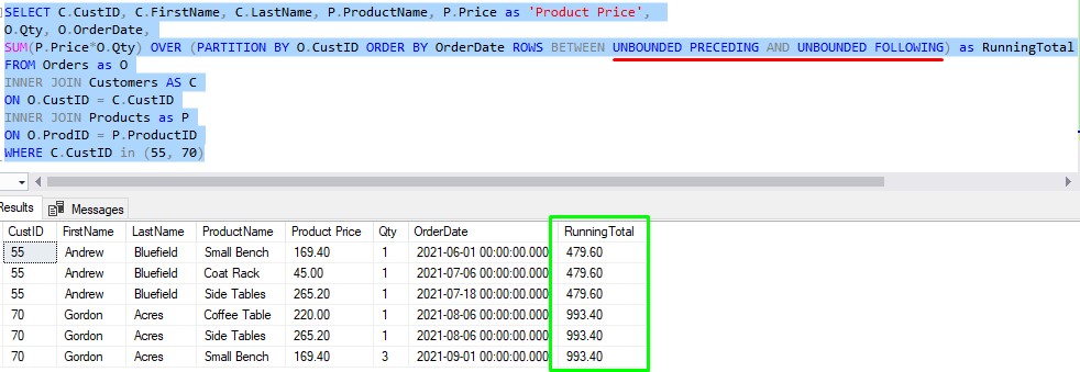
(It also includes the sum of the current row, in case you’re wondering. I think it’s because the word BETWEEN is inclusive, so it automatically includes the sum of the current row we’re looking at, too. For example, for the first row for Andrew Bluefield, the total sum will be everything before the first row (which is nothing), plus the current row (because the word BETWEEN is inclusive), plus everything after the current row in his window, giving us a grand total of $479.60)

Understand this would be silly to do, because it’s the same thing that would happen if we simply left out a frame completely. Remember this?:

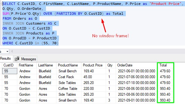
It’s the same result set.

I encourage you to play around with this. Instead of saying “UNBOUNDED“, experiment with saying “N PRECEDING | FOLLOWING“. Maybe something like ROWS BETWEEN 2 PRECEDING AND CURRENT ROW

Or even ROWS BETWEEN UNBOUNDED PRECEDING and 1 FOLLOWING

Play around with it, and double check the math. You’ll learn something new, I guarantee it!

Understanding the RANGE unit

I said earlier that there are two window units you can specify: ROWS or RANGE.

For example, in our SUM query, we can use the word RANGE instead of ROWS (and I’ll use that shorthand method I talked about earlier):

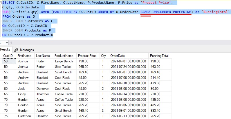
So, what’s the difference? Let’s isolate the rows for our customer Gordon Acres:

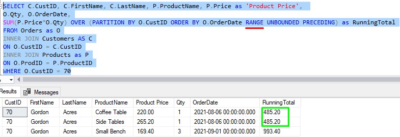
Notice the first two values for our RunningTotal column. They are the same, $485.20

Also notice how both those rows have the same OrderDate value, 8/6/2021

Now let’s look at the results if we use the ROWS unit instead:

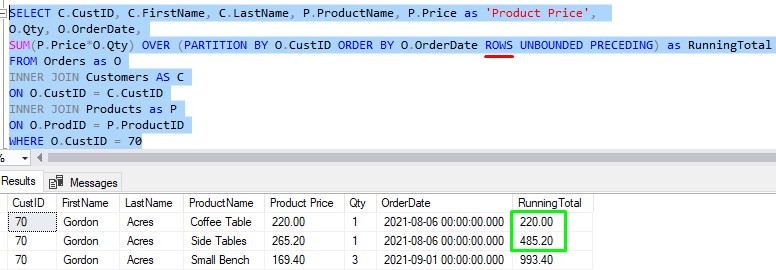
The RunningTotal values are more in-line with what we came up with earlier. But why?

The technical explanation for this is that the RANGE unit includes peers, while the ROWS unit does not.

A “peer” would be two or more rows that have the same ordering value.

Think about our window order clause, which is by OrderDate. A “peer” would be two or more rows that have the same OrderDate value.

For customer Gordon Acres, his first two rows do, in fact, have the same OrderDate value. RANGE is going to SUM the values in both rows while ROWS will SUM them one at a time.

I guess if you think about it, Gordon Acres did spend a total of $485.20 on that specific day. So maybe the use of RANGE is more appropriate. But really, it all depends on what you want to see.

Limitations of RANGE

As I mentioned earlier, the only frames supported with RANGE are the following:

• UNBOUNDED PRECEDING
• UNBOUNDED FOLLOWING
• CURRENT ROW

Basically, you can’t use the N PRECEDING | FOLLOWING frame with RANGE.

Also, Microsoft makes it clear that the RANGE unit is not as efficient as ROWS. So understand that if you must use it, your query may perform worse than if you were to use ROWS.

5. Tips, tricks, and links

Here is a list of some helpful tips and tricks you should know when working with window functions in SQL Server.

Tip # 1: Window functions can only be used in the SELECT list or ORDER BY clause.

Not much else to say. You can only use a window function in the SELECT list or an ORDER BY clause.

Tip # 2: If you specify a window order clause without a window frame clause, the frame will default to RANGE UNBOUNDED PRECEDING

Remember this window aggregate query we wrote earlier:

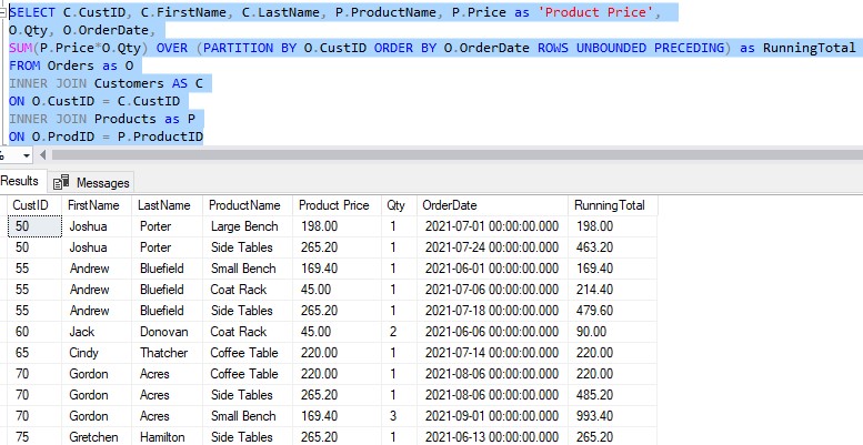
If you wanted to, you could leave out the frame completely. Like this:

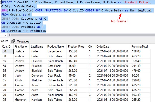
Understand that if you do this, a frame will be defaulted for you. The frame will be RANGE BETWEEN UNBOUNDED PRECEDING AND CURRENT ROW, otherwise known as RANGE UNBOUNDED PRECEDING for short.

Do you remember what I said about the RANGE unit? RANGE includes peers, while ROWS does not.

Also again, remember that RANGE is not as efficient as ROWS.

This leads nicely into our next tip…

Tip # 3: If you specify a window order clause, you really should specify your own window frame clause

With aggregate window functions, it’s honestly better to explicitly write the window frame you want to use. The only way I would NOT outline a frame is if I wanted to specifically use the frame RANGE UNBOUNDED PRECEDING. I know SQL will use this frame by default, so it would be redundant for me to outline it myself.

Links:

Everything discussed in this tutorial can be found in the following FREE Ebook:

Download your FREE SQL Server Window Functions EBook!

This Ebook discusses absolutely everything you need to know about window functions in SQL Server, including everything discussed in this tutorial. A proper understanding of window functions is essential for anyone looking to enter the field of data science. This eBook will definitely be a great resource for you to reference throughout your career. Get it today!

Next Steps:

Now that you understand aggregate window functions, and what window functions are in general, you should check out my full introduction to ranking window functions found here:

SQL Server Ranking Window Functions: ROW_NUMBER, RANK, DENSE_RANK, NTILE

If you want to be a great database developer, you should definitely be familiar with all the different window functions available in SQL Server.

Thank you very much for reading!

Make sure you subscribe to my newsletter to receive special offers and notifications anytime a new tutorial is released!

If you have any questions, or if you are struggling with a different topic related to SQL Server, I’d be happy to discuss it. Leave a comment or visit my contact page and send me an email!